Skip to content


Satellite data offer several advantages. They provide regional coverage, allowing geologists to see large structures that span tens or hundreds of kilometres. They are cost-effective, because many datasets are free or inexpensive compared with airborne surveys or large field campaigns. They enable rapid reconnaissance of remote or inaccessible terrain. They offer repeat coverage and multiple wavelengths that help distinguish rock types, vegetation, soil, and moisture. They also give a consistent base for compiling maps from different sources.
The limitation is that imagery shows the surface, not the subsurface, and surface expression can be masked by vegetation, soil, cloud, and human activity. Interpretation must therefore be treated as a hypothesis to be tested.
Main Data Sources
Optical multispectral imagery. Landsat 8 and 9 (30 metre resolution) and Sentinel-2 (10 to 20 metre resolution) are widely used, free, and cover the whole of Kenya. They record visible, near-infrared, and shortwave infrared bands that help distinguish rock and soil types, alteration minerals, and vegetation. ASTER imagery adds thermal and additional shortwave infrared bands useful for mineral mapping, although its shortwave sensor has limitations in data availability.
High-resolution commercial imagery. Sub-metre satellite images, available through commercial providers and some web mapping services, allow detailed mapping of fault scarps, veins, and outcrops, particularly at prospect scale.
Digital elevation models (DEMs). The Shuttle Radar Topography Mission (SRTM) and Copernicus DEM provide global elevation data at roughly 30 metre resolution, and ALOS and other products offer comparable or finer detail. DEMs are the single most valuable data for structural interpretation, as they reveal landforms regardless of vegetation colour or illumination.
Radar imagery. Sentinel-1 and ALOS PALSAR synthetic aperture radar (SAR) penetrate cloud and, to some extent, vegetation, highlighting surface roughness and moisture. L-band radar can reveal structures beneath dry cover or vegetation in some environments. Radar interferometry can detect small ground movements along active faults.
Geophysical gridded data. Although not satellite imagery in the strict sense, airborne magnetic and radiometric grids and satellite-derived gravity data are often interpreted alongside imagery to map structures beneath cover.
Image Processing Techniques That Reveal Structure
Raw images are rarely enough. Processing enhances structural features.
Hillshade and relief shading. Generating hillshaded relief from a DEM, with illumination from several azimuths (for example, 0, 45, 90, and 135 degrees), reveals lineaments in all orientations, since features parallel to the light direction are suppressed. Combining multiple hillshades or using slope and curvature maps reduces illumination bias.
Slope, aspect, and curvature analysis. Maps of slope steepness, direction, and curvature highlight scarps, ridge crests, and valley axes that trace faults and folds.
Contrast stretching and band combinations. Adjusting the display range and selecting band combinations, for example a false-colour composite using shortwave infrared, near-infrared, and red bands, helps distinguish rock units and vegetation patterns related to structure.
Principal component analysis (PCA). PCA condenses the information in many bands into a few uncorrelated components, enhancing subtle differences between rock types and highlighting contacts.
Band ratios. Ratios of selected bands can emphasise iron oxides, clays, and carbonates, supporting alteration mapping along shear zones and faults.
Spatial filtering and edge enhancement. Directional filters and edge detection highlight linear features. Automated lineament extraction algorithms can produce candidate lineaments quickly, though they need manual review.
Pan-sharpening and image fusion. Combining high-resolution panchromatic data with lower-resolution multispectral data sharpens details while preserving colour information.
Drainage analysis. Rivers and streams adjust to structure. Straight stream segments, sharp elbow bends, offset channels, and rectangular or trellis drainage patterns point to fault and joint control.
What Structures Look Like from Space
Faults. Look for straight or gently curved linear features, abrupt breaks in slope (scarps), linear valleys, offset ridges and streams, aligned springs or lakes, and juxtaposition of different landscape textures. In the Kenya Rift, fault scarps form distinctive step-like terrain on the rift floor and flanks, and are readily seen on DEM hillshades.
Folds. Folded layered rocks show curved outcrop patterns, with ridges forming arcs or closures at plunging fold noses. Repeating bands of colour or texture on both sides of an axis suggest anticlines and synclines. Dip slopes and escarpments show the orientation of layers.
Shear zones. In basement terrains, shear zones may appear as linear zones of changed texture, aligned valleys, or abrupt changes in structural grain. Curving and deflection of foliation trends into a linear zone, visible on aeromagnetic and imagery data, often indicates shearing.
Joints and fracture corridors. Parallel sets of closely spaced lineaments often reflect joint swarms. Fracture corridors can control drainage, vegetation lines, and groundwater occurrence.
Dykes. Straight, narrow ridges or trenches, or linear magnetic anomalies, can mark dykes cutting across other structures.
Circular and arcuate features. Rings and arcs may indicate intrusions, volcanic calderas, or domes, which relate to structural settings and mineralisation in some terrains.
A Practical Interpretation Workflow
1. Define objectives and scale. Decide what you need: regional structural framework, prospect-scale targets, or hazard mapping. This sets the imagery resolution and mapping scale.
2. Compile and prepare data. Gather imagery, DEMs, geological maps, geophysical data, and existing structural measurements. Reproject all datasets to a common coordinate system, such as WGS84 with UTM Zone 36 or 37 for Kenya. Mosaic images, correct for atmospheric effects where needed, and choose cloud-free scenes, ideally from the dry season.
3. Generate derived products. Produce multi-azimuth hillshades, slope and curvature maps, band composites, PCA images, and drainage networks.
4. Interpret systematically. Digitise lineaments and structural features in a GIS at a consistent scale, working across the whole area rather than focusing on a few obvious features. Use separate layers for different feature types, such as faults, folds, joints, dykes, and contacts. Record attributes such as confidence level, interpreted type, and the data source used.
5. Analyse orientation and density. Plot lineament orientations on rose diagrams, and compute density maps to find zones of intense fracturing and intersections of different trends. Cluster and intersection zones are often exploration targets or high-permeability areas.
6. Integrate with other data. Compare with geological maps, geophysics, geochemistry, and known mineral occurrences, boreholes, or hot springs. Look for correlations that raise confidence in the interpretation.
7. Validate in the field. Plan ground checks along representative lineaments, measure structures, and confirm or reject interpretations. Update the model based on field results.
8. Report with uncertainty. Present the interpretation with clear distinctions between observed, inferred, and speculative features.
Common Pitfalls and How to Avoid Them
Man-made linear features. Roads, railways, pipelines, fence lines, field boundaries, and power lines can be mistaken for faults. Overlay infrastructure layers and check high-resolution images to exclude them.
Illumination bias. Features perpendicular to the light direction are enhanced, while those parallel are hidden. Use multiple illumination angles.
Scale dependence. Lineaments may look continuous at one scale and fragmented at another. Document the scale used.
Over-interpretation. It is tempting to draw every faint linear feature. Prioritise lineaments with supporting evidence, such as offsets, geomorphic expression, or geophysical correlation.
Lithological and geomorphic confusion. Contacts between resistant and weak rocks, drainage divides, and river terraces can resemble structures. Use geological context and field checks.
Vegetation and soil cover. Dense forest, cropland, and thick soils in parts of Kenya can obscure bedrock. In such areas, radar, DEMs, and geophysics are more useful than optical imagery.
Seasonal and cloud effects. Cloud, haze, and seasonal vegetation changes alter image appearance. Use multi-temporal data and choose scenes carefully.
Not all lineaments are faults. A lineament is a surface pattern, not a proven geological structure. Always call them lineaments until validated.
Applications in Kenya
Mineral exploration. Structural interpretation helps outline shear corridors and fault intersections in the greenstone belts of western Kenya and the Mozambique Belt, guide soil sampling lines, and prioritise ground for field mapping. Alteration mapping from multispectral data can complement structural targets.
Geothermal exploration. In the Rift Valley, mapping fault patterns, fissures, and volcanic alignments from imagery and DEMs helps identify permeable zones, accommodation zones, and prospective areas.
Hydrogeology. Fracture traces and lineament intersections in crystalline basement and volcanic terrains help siting boreholes, as they often indicate zones of enhanced groundwater storage and flow.
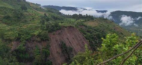
Engineering and hazards. Mapping fault scarps, landslide scars, and unstable slopes from imagery supports infrastructure routing, dam siting, and hazard zonation.
Regional geological mapping. Imagery assists in extending mapped boundaries into poorly exposed areas and checking older maps.
Software and Skills
Common tools include QGIS (free and open source), ArcGIS, ENVI, ERDAS, PCI Geomatica, and cloud platforms such as Google Earth Engine for large-scale processing. Interpreters benefit from training in structural geology, remote sensing principles, and GIS, as well as familiarity with the local geology. Collaboration between remote sensing specialists and field geologists leads to the best results.
Frequently Asked Questions
Can satellite imagery replace field mapping? No. It guides and supplements field mapping, but rock description, structural measurement, and sampling still require ground observation.
Which imagery is best for structure? DEMs and hillshades are generally the most valuable, supported by multispectral and radar data.
How accurate are interpreted lineaments? Accuracy depends on resolution, geology, and interpreter skill. Field validation is essential.
Conclusion
Satellite imagery has transformed structural geology by giving geologists a regional view of faults, folds, shear zones, and fracture systems before the first field traverse. By combining DEMs, multispectral and radar data, careful processing, systematic interpretation, and rigorous field validation, explorers and engineers in Kenya can build reliable structural frameworks quickly and economically. The key is to treat the interpretation as a living model, refined with every new piece of evidence from the ground.